Monday 8 August 2016

GBIF Backbone - August 2016 Update

GBIF has just put a new backbone taxonomy into production! Since our last update of the GBIF Backbone we have received various feedback and gained insight into potential code improvements. Here is a quick summary of what has changed in this August 2016 version.

Important code changes:

  • much less eager basionym detection resulting in fewer algorithmically assigned synonyms and removing many false synonyms especially in plants
  • detect and merge orthographic variants of species doing gender stemming, allowing double consonant characters, deal with author transliterations and merging hybrid names

All fixed issues in the source code that generates a new backbone can be found there, each of them often leads to actual reported user feedback: http://dev.gbif.org/issues/browse/POR-3029

New sources

The following new sources have been incorporated into the august backbone:
  • major new version of The Paleobiology Database contributing 2,315 new families, 11,390 genera and 131,958 species names to the backbone. Feeds many isExtinct and livingPeriod values into the backbone for fossil taxa
  • thousands of new Plazi articles with 1,883 genera, 28,725 species and 1,935 infraspecific names. Only use genus names and below from Plazi, excluding any synonyms until we are confident they are all correctly marked up
  • added Artsnavnebasen source, contributing 3,640 new genera and 29,751 species names to the backbone
  • added International Cichorieae Network source, contributing 190 new Asteraceae genera; 1,415 species and 3,427 infraspecies names to the backbone
The 39 sources used in this backbone build

Backbone impact

The new backbone has a total of 5,307,978 names of which it treats 2,525,274 species names as accepted (previously 2,420,842 out of 5,208,172). More backbone metrics are available through our portal and in more detail through our API.
  • 187,854 deleted names, mostly due to the removal of orthographic variants
  • 279,404 new names 
    • Unknown: 165 families; 743 genera; 785 species; 14 infraspecific
    • Animalia: 13 order; 1,649 families; 10,171 genera; 125,478 species; 4,398 infraspecific
    • Archaea: 2 genera; 3 species
    • Bacteria: 1 families; 33 genera; 544 species; 36 infraspecific
    • Chromista: 38 families; 412 genera; 5,594 species; 295 infraspecific
    • Fungi: 1 families; 691 genera; 11,127 species; 2,039 infraspecific
    • Plantae: 50 families; 666 genera; 82,672 species; 14,725 infraspecific
    • Protozoa: 1 class; 1 order; 4 families; 38 genera; 349 species; 24 infraspecific
    • Viruses: 1 families; 982 genera; 6,311 species
A very large and detailed log of the backbone build is also available.

The largest taxonomic groups in the backbone, exceeding 3% of all accepted species is shown in the following diagram:


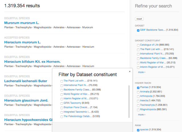
The Catalogue of Life as the largest single primary source contributes 59,8% of all names (previously 60,9%). A breakdown by backbone constituents is now also available as a species search facet. For example this shows the breakdown for all accepted plant species in the backbone:


Occurrence impact

With a new backbone we have reprocessed all of our 642 million occurrences. The larger changes were:
  • Fixed various old/new world distributions of incorrectly synonymized species
  • Reduced the number of virus records from 157,492 down to just 5,348 records. Most occurrences were Lepidoptera, e.g. the common peacock butterfly that had formerly been mismatched because there was no classification given with the name.
Some more metrics of backbone names in our occurrences. There are:
  • 216,699 distinct genera in GBIF occurrences. That is 55% out of all 396.990 genera in the backbone
  • 1,226,668 accepted species in GBIF occurrences. That is 50% out of all 2,420,842 backbone species
  • 2,059,961 distinct names in GBIF occurrences. Which is 39% of all 5.208.172 names in the backbone
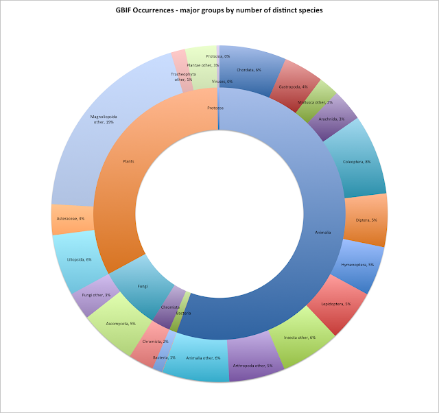
The distribution of the major taxonomic groups exceeding 3%, i.e have a minimum of 36.800 species, is shown in this last diagram:


Wednesday 20 July 2016

Probably Turboveg's best-kept secret

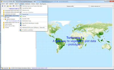
Turboveg is one of the most widely used software programs used to manage vegetation data. Probably its best-kept secret is that it can export vegetation data in Darwin Core Archive (DwC-A) format, which is a standard format that enables its quick and easy integration with other resources on GBIF.org. Turboveg v2 converts vegetation data into species occurrence data packaged as a DwC-A. Now thanks to an 8 month long collaboration between GBIF and Stephan Hennekens (Turboveg's developer), v3 will convert vegetation data into sampling event data packaged as a DwC-A - a much more faithful and useful representation of the data.

Turboveg

Screenshot of Turboveg v3 prototype
Turboveg is an easy to install and easy to use Windows program for storing, managing, visualizing and exporting vegetation data (relevés). A relevé is a list of the plants in a delimited plot of vegetation, with information on species cover and on substrate and other abiotic features in order to make as complete as possible description in terms of plant community composition and structure.

Today there are about 1500 users of the software worldwide managing more than 1,5 million relevés. Turboveg can export relevés in various file formats, which is useful to enable further analysis. Support for exporting relevés as species occurrence data packaged as a Darwin Core Archive (DwC-A) was added to v2 in 2011. Guidance on how to use this feature can be found in the Turboveg User Manual.

Version 3, due to be released in 2017, will export relevés as sampling event data packaged as DwC-A - a format that more accurately reflects the original data.

Sampling event data

Sampling event data derive from environmental, ecological, and natural resource investigations that follow standardized protocols for measuring and observing biodiversity. This is in contrast to opportunistic observation and collection data, which today form a significant proportion of openly accessible biodiversity data. A good example of sampling data is data coming from vegetation sampling events using the Braun-Blanquet protocol. Because the sampling methodology and sampling units are precisely described the resulting data is comparable and thus better suited for measuring trends in habitat change and climate change.

Sampling event data model

A data model provides the details of the structure of the data. Previously sampling event data couldn't be modelled in a standardized way in Darwin Core due to the complexity of encoding the underlying protocols. Over the past two years, however, GBIF has been working with EU BON and the wider bioinformatics community to develop a data model for sharing sampling event data. In March 2015 TDWG, the international body responsible for maintaining standards for the exchange of biological data, ratified changes that enabled support for modelling sampling event data.

In summary, the de facto data model for sampling event data in Darwin Core consists of three tables: Sampling event, Measurements or Facts and Species occurrences. 

A Sampling event can be associated with many Species occurrences, while a Species occurrence can only be associated to one Sampling event. Similarly, a Sampling event can be associated with many Measurements or Facts. In this way a Sampling event has a one-to-many relationship to both Species occurrences and Measurements or Facts. 

Note additional tables of information can also be added to a Sampling event, such as Multimedia (e.g. to record images of the plot). More information about this preferred data model for sampling event data can be found in the IPT Sampling Event Data Primer.


Sampling event data model for vegetation plot data

Vegetation surveys or relevés produce a wealth of information on species cover and on substrate and other abiotic features in the plot. Species cover can be measured using dozens of different vegetation abundance scales such as the Braun-Blanquet scale or Londo decimal scale to name a couple. To standardize how this information is stored, a custom Relevé table is used instead of the Measurements or Facts table.

This data model for vegetation plot data in Darwin Core consists of three tables: Sampling event, Relevé and Species Occurrence.

A Sampling event can be associated with only one Relevé. The Relevé consists of the most common relevé measurements covering all vegetation layers. Note for each measurement the unit and precision is explicitly defined. A Sampling event can also be associated with many Species occurrences, however, each Species occurrence should specify the vegetation layer where it was found hence the same species can be found within multiple vegetation layers. In this way the vegetation composition can be described for each layer within the plot.

Note that at the time of writing the Darwin Core standard doesn't have the terminology for storing vegetation layers. Therefore a formal proposal has been made to add the new term "layer" to Darwin Core. To standardise how this new term is populated, a custom vocabulary for vegetation layers has also been produced.


Example DwC-A export by Turboveg: Dutch Vegetation Database (LVD)

Fortunately, the Dutch Vegetation Database (LVD) has recently been republished using the new sampling event format and can thus serve as an exemplar dataset. LVD is a substantial dataset published by Alterra (a major Dutch research institute) that covers all plant communities in the Netherlands with more than 85 years of vegetation recording for some habitats. The latest version of this dataset has more than 650 thousand relevés associated with almost 12 million species occurrences.

Alterra uses Turboveg v3 to manage this dataset and export it in the standardized DwC-A format. It is important to note that special care is taken by the software to protect sensitive species: the location of plots, which have red list species observed in them, are obfuscated to a level of 5x5 km squares. Furthermore the software converts all coverage values to the same unit (e.g. species coverage values are converted into percentage coverage) in order to make the data easy to use and integrate with other sources.

Sampling event data on GBIF.org: Dutch Vegetation Database (LVD)

GBIF.org map of LVD georeferenced data
All versions of LVD are imported to the EU BON IPT where they get archived and published through GBIF.org

The 8 month long collaboration between GBIF and Stephan Hennekens culminated in the latest version of LVD being indexed into GBIF.org here. A special and grateful thanks is owed to Stephan for all his hard work to make this happen.

Over the next couple of years GBIF will continue working on enhancing the indexing and discovery of sampling event datasets (e.g. showing events' plots/transects on a map, filtering events by sampling protocol, indexing Relevés, etc.). At least when Turboveg v3 is released in 2017, users can already export their relevés into this new standardized format that represents their data much more faithfully.

Wednesday 6 April 2016

Updating the GBIF Backbone

The taxonomy employed by GBIF for organising all occurrences into a consistent view has remained unchanged since 2013. We have been working on a replacement for some time and are pleased to introduce a preview in this post. The work is rather complex and tries to establish an automated process to build a new backbone which we aim to run on a regular, probably quarterly basis. We would like to release the new taxonomy rather soon and improve the backbone iteratively. Large regressions should be avoided initially, but it is quite hard to evaluate all the changes between 2 large taxonomies with 4 - 5 million names each. We are therefore seeking feedback and help to discover oddities of the new backbone.

Relevance & Challenges

Every occurrence record in GBIF is matched to a taxon in the backbone. Because occurrence records in GBIF cover the whole tree of life and names may come from all possible, often outdated, taxonomies, it is important to have the broadest coverage of names possible. We also deal with fossil names, extinct taxa and (due to advanced digital publishing) even names that have just been described a week before the data is indexed at GBIF.
The Taxonomic Backbone provides a single classification and a synonymy that we use to inform our systems when creating maps, providing metrics or even when you do a plain occurrence search. It is also used to crosslink names between different checklist datasets.

The Origins

The very first taxonomy that GBIF used was based on the Catalogue of Life. As this only included around half the names we found in GBIF occurrences, all other cleaned occurrence names were merged into the GBIF backbone. As the backbone grew we never deleted names and increasingly faced more and more redundant names with slightly different classifications. It was time for a different procedure.

The Current Backbone

The current version of the backbone was built in July 2013. It is largely based on the Catalogue of Life from 2012 and has folded in names from 39 further taxonomic sources. It was built using an automated process that made use of selected checklists from the GBIF ChecklistBank in a prioritised order. The Catalogue of Life was still the starting point and provided the higher classification down to orders. The Interim Register of Marine and Nonmarine Genera was used as the single reference list for generic homonyms. Otherwise only a single version of any name was allowed to exist in the backbone, even where the authorship differed.

Current issues

We kept track of nearly 150 reported issues. Some of the main issues showing up regularly that we wanted to address were:
  • Enable an automated build process so we can use the latest Catalogue of Life and other sources to capture newly described or currently missing names
  • It was impossible to have synonyms using the same canonical name but with different authors. This means Poa pubescens was always considered a synonym of Poa pratensis L. when in fact Poa pubescens R.Br. is considered a synonym of Eragrostis pubescens (R.Br.) Steud.
  • Some families contain far too many accepted species and hardly any synonyms. Especially for plants the Catalogue of Life was surprisingly sparsely populated and we heavily relied on IPNI names. For example the family Cactaceae has 12.062 accepted species in GBIF while The Plant List recognizes just 2.233.
  • Many accepted names are based on the same basionym. For example the current backbone considers both Sulcorebutia breviflora Backeb. and Weingartia breviflora (Backeb.) Hentzschel & K.Augustin as accepted taxa.
  • Relying purely on IRMNG for homonyms meant that homonyms which were not found in IRMNG were conflated. On the other hand there are many genera in IRMNG - and thus in the backbone - that are hardly used anywhere, creating confusion and many empty genera without any species in our backbone.

The New Backbone

The new backbone is available for preview in our test environment. In order to review the new backbone and compare it to the previous version we provide a few tools with a different focus:
  • Stable ID report: We have joined the old and new backbone names to each other and compared their identifiers. When joining on the full scientific name there is still an issue with changing identifiers which we are still investigating.
  • Tree Diffs: For comparing the higher classification we used a tool from Rod Page to diff the tree down to families. There are surprisingly many changes, but all of them stem from evolution in the Catalogue of Life or the changed Algae classification.
  • Nub Browser: For comparing actual species and also reviewing the impact of the changed taxonomy on the GBIF occurrences, we developed a new Backbone Browser sitting on top of our existing API (Google Chrome only). Our test environment has a complete copy of the current GBIF occurrence index which we have reprocessed to use the new backbone. This also includes all maps and metrics which we show in the new browser.
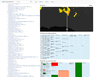
Family Asparagaceae as seen in the nub browser:
Red numbers next to names indicate taxa that have fewer occurrences using the new backbone, while green numbers indicate an increase. This is also seen in the tree maps of the children by occurrences. The genus Campylandra J.G. Baker, 1875 is dark red with zero occurrences because the species in that genus were moved into the genus Rhodea in the latest Catalog of Life.

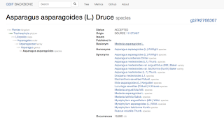
Species Asparagus asparagoides as seen in the nub browser:
The details view shows all synonyms, the basionym and also a list of homonyms from the new backbone.

Sources

We manually curate a list of priority ordered checklist datasets that we use to build the taxonomy. Three datasets are treated in a slightly special way:
  1. GBIF Backbone Patch: a small dataset we manually curate at GBIF to override any other list. We mainly use the dataset to add missing names reported by users.
  2. Catalogue of Life: The Catalogue of Life provides the entire higher classification above families with the exception of algaes.
  3. GBIF Algae Classification: With the withdrawal of Algaebase the current Catalogue of Life is lacking any algae taxonomy. To allow other sources to at least provide genus and species names for algae we have created a new dataset that just provides an algae classification down to families. This classification fits right into the empty phyla of the Catalogue of Life.
The GBIF portal now also lists the source datasets that contributed to the GBIF Backbone and the number of names that were used as primary references.

Other Improvements

As well as fixing the main issues listed above, there is another frequently occurring situation that we have improved. Many occurrences could not be matched to a backbone species because the name existed multiple times as an accepted taxon. In the new backbone, only one version of a name is ever considered to be accepted. All others now are flagged as doubtful. That resolves many issues which prevented a species match because of name ambiguity. For example there are many occurrences of Hyacinthoides hispanica in Britain which only show up in the new backbone (old / new occurrence, old / new match). This is best seen in the map comparison of the nub browser, try to swipe the map!

Known problems

We are aware of some problems with the new backbone which we like to address in the next stage. Two of these issues we consider as candidates for blocking the release of the new backbone:
Species matching service ignores authorship
As we better keep different authors apart the backbone now contains a lot more species names which just differ by their authorship. The current algorithm only keeps one of these names as the accepted name from the most trusted source (e.g. CoL) and treats the other as doubtful if they are not already treated as synonyms.
The problem currently is that the species matching service we use to align occurrences to the backbone does not deal with authorship. Therefore we have some cases where occurrences are attached to a doubtful name or even split across some of the “homonyms”.
There are nearly 166.832 species names with different authorship existing in the new backbone, accounting for 98.977.961 occurrences.
Too eager basionym merging
The same epithet is sometimes used by the same author for different names in the same family. This currently leads to an overly eager basionym grouping with less accepted names.
As these names are still in the backbone and occurrences can be matched to them this is currently not considered a blocker.

Thursday 25 February 2016

Reprojecting coordinates according to their geodetic datum

For a long time Darwin Core has a term to declare the exact geodetic datum used for the given coordinate. Quite a few data publishers in GBIF have used dwc:geodeticDatum for some time to publish the datum of their location coordinates.

Until now GBIF has treated all coordinates as if they were in WGS84, the widespread global standard datum used by the Global Positioning System (GPS). Accordingly locations given in a different datum, for example NAD27 or AGD66, were displaced on GBIF maps a little. This so called “datum shift” is not dramatic, but can be up to a few hundred metres depending on the location and datum. The Univeristy of Colorado has a nice visualization of the impact.

At GBIF we interpret the geodeticDatum and reproject all coordinates as good as we can into the single datum WGS84. In order to do this there are two main steps that need to be done: parse and interpret the given verbatim geodetic datum and then do the actual transformation based on the known geodetic parameters.

Parsing geodeticDatum

As usual GBIF receives a lot of noise when reading the dwc:geodeticDatum. After removing the obvious bad values, e.g. introduced by bad mappings done by the publisher, we still ended up with over 300 different values for some datum. Most commonly simple names or abbreviations are used, e.g. NAD27, WGS72, ED50, TOKYO. In some cases we also see proper EPSG http://www.epsg.org/ codes coming in, e.g. EPSG:4326 which is the EPSG code for WGS84. As EPSG is a widespread and complete reference dataset of geodetic parameters, supported by many java libraries, we decided to add a new DatumParser to our parser library that directly returns EPSG integer codes for datum values. That way we can lookup geodetic parameters easily in the following transformation step. In addition to parse any given EPSG:xyz code directly it also understands most datums found in the GBIF network based on a simple dictionary file which we manually curate.

Even though EPSG codes are well maintained, very complete and supported by most software opaque integer codes have a harder time to get used than meaningful short names. Maybe a lesson we should keep in mind when debating about identifiers elsewhere.

Our recommendation to publishers is to use the EPSG codes if you know them, otherwise stick to the simple well known names. A good place to search for EPSG codes is http://epsg.io/.

Transformation

Once we have a decimal coordinate and a well known geodetic source datum the transformation itself is rather straight forward. We use geotools to do the work. The first step in the transformation is to instantiate a CoordinateReferenceSystem (CRS) using the parsed EPSG code of the geodeticDatum. A CRS combines a datum with a coordinate system, in our case this always a 2 dimensional system with the prime meridian in Greenwich and longitude values increasing East, latitude values North.

As EPSG codes can refer to both, just a plain datum and also a complete spatial reference system, we need to take this into account when building the CRS like this:

 private CoordinateReferenceSystem parseCRS(String datum) {
    CoordinateReferenceSystem crs = null;
    // the GBIF DatumParser in use
    ParseResult<Integer> epsgCode = PARSER.parse(datum);
    if (epsgCode.isSuccessful()) {
      final String code = "EPSG:" + epsgCode.getPayload();
      // first try to create a full fledged CRS from the given code
      try {
        crs = CRS.decode(code);

      } catch (FactoryException e) {
        // that didn't work, maybe it is *just* a datum
        try {
          GeodeticDatum dat = DATUM_FACTORY.createGeodeticDatum(code);
      // build a CRS using the standard 2-dim Greenwich coordinate system
          crs = new DefaultGeographicCRS(dat, DefaultEllipsoidalCS.GEODETIC_2D);

        } catch (FactoryException e1) {
          // also not a datum, no further ideas, log error
          LOG.info("No CRS or DATUM for given datum code >>{}<<: {}", datum, e1.getMessage());
        }
      }
    }
    return crs;
  }

Once we have a CRS instance we can create a specific WGS84 transformation and apply it to our coordinate:

public ParseResult<LatLng> reproject(double lat, double lon, String datum) {
   CoordinateReferenceSystem crs = parseCRS(datum);
   MathTransform transform = CRS.findMathTransform(crs, DefaultGeographicCRS.WGS84, true);
   // different CRS may swap the x/y axis for lat lon, so check first:
   double[] srcPt;
   double[] dstPt = new double[3];
   if (CRS.getAxisOrder(crs) == CRS.AxisOrder.NORTH_EAST) {
     // lat lon
     srcPt = new double[] {lat, lon, 0};
   } else {
     // lon lat
     srcPt = new double[] {lon, lat, 0};
   }

   transform.transform(srcPt, 0, dstPt, 0, 1);
   return ParseResult.success(ParseResult.CONFIDENCE.DEFINITE, new LatLng(dstPt[1], dstPt[0]), issues);
  }

The actual projection code does a bit more of null and exception handling which I have removed here for simplicity.

As you can see above we also have to watch out for spatial reference systems that use a different axis ordering. Luckily geotools knows all about that and provides a very simple way to test for it.

Issue flags

As with most of our processing we flag records when problems or assumed behavior occurs. In the case of the geodetic datum processing we keep track of 5 distinct issues which are available as GBIF portal occurrence search filters:

  • COORDINATE_REPROJECTION_FAILED: A CRS was instantiated, but the transformation failed for some reason.
  • GEODETIC_DATUM_INVALID: The datum parser was unable to return an EPSG code for the given datum string.
  • COORDINATE_REPROJECTION_SUSPICIOUS: The reprojection resulted in a datum shift larger than 0.1 degrees.
  • GEODETIC_DATUM_ASSUMED_WGS84: No datum was given or the given datum was not understood. In that case the original coordinates remain untouched.
  • COORDINATE_REPROJECTED: The coordinate was successfully transformed and differs now from the verbatim one given.